Regression Analysis

Regression analysis is a method to define the mathematical relationship between an output variable (y) and one or more input variable (x1, x2,….etc.) This mathematical relationship or equation is called the regression model.

Basically, the regression model is an equation that can be used to predict the value of ‘y’ using the input variables i.e. ‘y’ expressed as a function of x1, x2…etc.

In order to understand a regression model, we start with a simple linear regression model. Here we find the relationship between the output variable and a single input variable.

Linear Regression Model

The regression model is y = b0 + b1x + S, where

• y = output variable, also known as dependent variable


• b0 = constant or coefficient of constant. Graphically, this is the y-intercept or the value of y when x = 0
  
• b1 = coefficient of x i.e. the slope or rate of change of y for a unit change of x


• x = input variable. X, along with the constant is also known as predictor since they are used to predict the value of y. It is also called the independent variable.


• S = error or residual value. I.e. it is the difference between the actual value of y and the value of y predicted by the regression model.

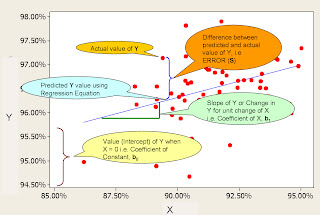
FIGURE 1: Regression Chart

Understanding the Regression Model

The regression model is better defined and understood using the regression model parameters. Let’s take the result of a regression analysis in Minitab.

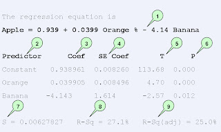
FIGURE 2: Regression Equation

1. The first line is the regression equation where y is predicted as a function of x
   
2. Predictor – x and the constant are the predictors used to predict the value of y


3. Coefficient – the value of b0 and b1, i.e. the coefficients of constant and x. The size of the coefficient is a measure of the magnitude of the influence of that predictor on y and the sign (+ve or –ve) of the coefficient shows the direction of the influence.


4. SE Coefficient – It is the Standard Error of the coefficient and is an estimate of the standard deviation of the coefficient. This is the precision with which the coefficients are calculated. The SE coefficient by itself doesn’t shed much light into the strength of the model. This is used in the t-test of the regression model to check the strength of the model. We check the strength of the model using the results of the t-test.


5. T-value – T-value if coefficient divided by the SE coefficient. Just like the SE coefficient, the T-value by itself does not tell us much about the strength of the model. The T-value is compared with values in the Student’s T Distribution to determine the P-value of the model. The Student’s T Distribution describes how the mean of a sample with n observations is expected to behave. The P-value is a measure of the strength of the model.


6. P-value – If 95% if the Students t distribution is closer to the mean than the T-value, of the coefficient, then the P-value of the coefficient is 5%. The P-value is the probability of seeing a similar result as ours in a random sample of the same size where the predictor has no influence on y. In simple terms, the P-value is the probability that the effect of the predictor on y occurred by a random chance i.e. the probability that the predictor has no real influence on y. It is generally accepted that if the P-value if 5% or less, we can reject this notion and conclude that the predictor has influence on y. A P-value of 5% (0.05) or less means that there is only a 5% chance that the results we are seeing is due to a random chance, i.e. there is a 95% chance that the predictor has influence on y. It is important to note that the P-value only shown the presence of a relationship and is not a measure of the magnitude of the relationship.


7. S – S is the residual or error of the regression equation. This is the difference between the predicted and the actual value of y i.e. an estimate of the standard deviation of the regression equation. Graphically, it is the variation of points around the regression line. S is also known as the sum of squares. The lower the value of S, the better the regression equation.


8. R-Sq measures the goodness of fit of the regression equation. This measures how well the predictors are able to predict the value of y. R-Sq ranges from zero (poor predictor) to one (perfect predictor). Basically the R-Sq value is the fraction of variation in y that can be predicted by the predictors. It is also known as the coefficient of determination. R-Sq of 1 does not occur in real life situations. The accepted value for R-Sq varies by situation, but 0.4 is generally considered an acceptable level.


9. Adjusted R-Sq. Adjusted R-Sq is similar to R-Sq, but it standardizes the value of R-Sq by taking into account the number of predictors involved in the equation. Generally, the larger the number of predictors, the stronger the regression model and R-Sq increases. Adjusted R-Sq modifies the R-Sq and makes it independent of the number of predictors involved. This makes it easier to compare one regression model to another.

Checking if the regression model is good enough

The two key parameters on checking the goodness of the Regression model are P-value of each predictor and R-Sq (or adjusted R-Sq) of the equation.

P-value shows the statistical significance of each predictor. If the P-value is greater than 0.05 for any predictor, it means that the variable has no significance on y. The insignificant variables should be removed from the regression model and the regression should be redone.

R-Sq shows how well the regression equation can predict the value of y.